0%

『论文笔记』Attention Consistency on Visual Corruptions for Single-Source Domain Generalization

Information

  • Title: Attention Consistency on Visual Corruptions for Single-Source Domain Generalization
  • Author: Ilke Cugu, Massimiliano Mancini, Yanbei Chen, Zeynep Akata
  • Institution: 作者单位不知道
  • Year: 2022
  • Journal: IEEE Computer Vision and Pattern Recognition Workshops (CVPRW), 2022
  • Source: OpenAccess, Arxiv, OfficialCode
  • Cite: Ilke Cugu, Massimiliano Mancini, Yanbei Chen, Zeynep Akata; Proceedings of the IEEE/CVF Conference on Computer Vision and Pattern Recognition (CVPR) Workshops, 2022, pp. 4165-4174
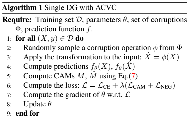
  • Idea: 原图与腐蚀图像的 CAM 图应该一致,即注意力集中在相同区域
1
2
3
4
5
6
7
8
@InProceedings{Cugu_2022_CVPR,
author = {Cugu, Ilke and Mancini, Massimiliano and Chen, Yanbei and Akata, Zeynep},
title = {Attention Consistency on Visual Corruptions for Single-Source Domain Generalization},
booktitle = {Proceedings of the IEEE/CVF Conference on Computer Vision and Pattern Recognition (CVPR) Workshops},
month = {June},
year = {2022},
pages = {4165-4174}
}

Abstract

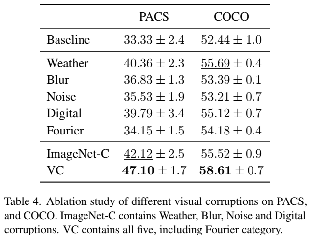
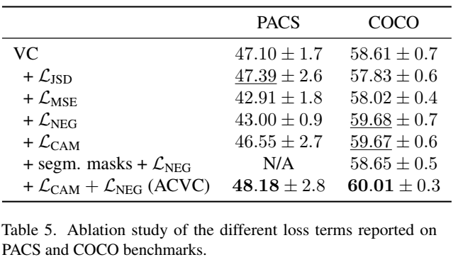
通过改变训练图像来模拟新的域,并对同一样本的不同视图添加一致性注意力。作者将该方法命名为视觉腐蚀的注意力一致性(Attention Consistency on Visual Corruptions, ACVC)

Introduction

通过使用多个合成的域进行训练使得模型能更好的分离域相关和语义相关的信息,消除模型预测与图像之间不正确的相关性,作者在此基础上提出,鲁棒的模型对于相同训练图像的不同数据增强视图应该有相同的语义表达,作者对原始样本和增强样本计算类激活映射(Class Activation Maps),并施加一致性约束,使其在特征空间的位置保持一致。

VisCo_teaser

另一方面,数据增强也很重要,上述任务要求数据增强能极大地改变输入图像但不会影响语义的空间位置,这篇文章中作者选择了天气、模糊、噪声、数字、傅里叶变换(去除低频、修改振幅、缩放相位)对样本进行增强。

该文章的贡献有:

  1. 分析视觉腐蚀作为单源域泛化的应用,包含 ImageNet-C 的19 种变换和 3 种基于傅里叶变换
  2. 提出了一种新的基于类激活映射的一致性损失来强制模型对于原样本和腐蚀样本查看相同区域
  3. 提出了新的单源域泛化基准测试,用在三个数据集
  4. 效果很好

Method

VisCo_flow

  1. 随机从 22 种增强(来自 ImageNet-C 和基于傅里叶变换)中采样
  2. 训练使得腐蚀图像和原图像 CAM 具有视觉一致性
  3. 通过负 CAM 损失最小化对 CAMs 进行正规化

整体目标函数为: \[ \mathcal{L}=\sum_{(X, y) \in \mathcal{D}} \mathcal{L}_{\mathrm{CE}}(X, \phi(X), y)+\lambda \mathcal{L}_{\mathrm{CON}}(X, \phi(X), y) \] 其中 \(\phi\) 是数据增强函数,\(\mathcal{L}_{\mathrm{CE}}\) 是交叉熵损失,\(\mathcal{L}_{\mathrm{CON}}\) 是一致性约束 \[ \mathcal{L}_{\mathrm{CE}}(X, \hat{X}, y)=-\log f_{\theta}^{y}(X)-\log f_{\theta}^{y}(\hat{X}), \]

Visual Corruptions

视觉腐蚀有两个来源:ImageNet-C 和 基于傅里叶的视觉腐蚀

ImageNet-C视觉腐蚀

包含 4 类 19 种 5 个级别的视觉腐蚀,4 中类型分别是:天气、模糊、噪音和数字,如上图所示

天气模拟气象障碍,如雾,雪,霜冻和飞溅,而模糊平滑图像像素的强度使用不同的功能,如高斯,玻璃,运动,散焦和缩放。噪声随机扰动像素值,使用不同的函数,即射击,脉冲,高斯和散斑,而数字收集由修改图像分辨率(即JPEG压缩,像素化,弹性)或像素强度(即饱和度,亮度和对比度)引起的各种损坏。

基于傅里叶的视觉腐蚀

已有的研究表明,图像的傅里叶变换中的相位保留了大部分语义信息,振幅主要保留了纹理信息。下面用 \(\mathcal{F}(X)\) 表示对图像进行傅里叶变换, \(\mathcal{F}^{-1}\) 表示逆傅里叶变换, \(\mathcal{F}^A(X)\) 表示振幅、 \(\mathcal{F}^P(X)\) 表示相位。

相位缩放:使用 \(\alpha \in (0, 1]\) 对相位进行缩放(上图第一个) \[ \phi_\text{P-scaling}(X) = \mathcal{F}^{-1}([\mathcal{F}^A(X),\alpha \mathcal{F}^P(X)]) \] 常数振幅:将振幅固定为 \(\beta \in (0, 1]\) 的常数(上图第二个) \[ \phi_\text{constant-A}(X) = \mathcal{F}^{-1}([\beta, \mathcal{F}^P(X)]) \] 高通滤波:通过在频谱图调整直径 \(d\) 过滤掉低频成分(上图第三个) \[ \phi_\text{high-pass}(X) = \mathcal{F}^{-1}(H^d(\mathcal{F}(X)) \circ \mathcal{F}(X))) \] 其中 \(H^d(F)\) 是滤波掩码 \[ H_{u,v}^d(F) = \begin{cases} 1, & \text{if} \;\;\; F_{u,v}\geq d\\ 0, & \text{otherwise.}\end{cases} \]

注意力一致性

基本出发点是无论图像如何变换,模型都应该关注图像的相同区域

CAMs 可视化特征图中对输出贡献最大的区域: \[ M = \sigma(W^\intercal g(X)) \] 其中 \(M\) 表示 CAM 图,\(g\) 表示特征提取器,\(W\) 是线性分类器,\(\sigma\) 表示 softmax 操作 \[ \sigma(x)^c_i = \frac{exp(x^c_i / T)}{\sum_{j=1}^{s}exp(x^c_j / T))} \] 作者提出的注意力一致性约束为: \[ \mathcal{L}_{\text{CAM}}(M,\hat{M},y) = D_{JS}(M_y || \hat{M}_y) \] 其中 \(\hat{M_y}\) 表示腐蚀图像对于分类标签 \(y\) 对应的 CAM 图,JS 散度也可以换成其他的目标函数,但实验中作者发现 JS 散度 (JSD) 比 MSE 损失更好。此外还能定义 softmax 的温度 \(T\) 来控制更灵活的目标, \(T < 1\) 只保留极端注意力区域,$T > 1 $ 是 CAM 图更平滑。

负 CAM 损失:由于这种方法高度依赖 CAM ,而 CAM 存在的一个问题是倾向于产生错误激活,所以提出使用负 CAM 损失来减少对错误类的注意力映射: \[ \mathcal{L}_{\text{NEG}}(M,C_k) = \sum_{c \in C_k} D_{KL}(U || M_c) + D_{KL}(U || \hat{M}_c), \] 其中 \(U\) 是均匀分布,\(C_k\) 是在干净图像 \(X\) 的置信度分数方面的前 \(k\) 负类的集合。

最终的目标函数为: \[ \mathcal{L} = \mathcal{L}_{\text{CE}} + \lambda (\mathcal{L}_{\text{CAM}} + \mathcal{L}_{\text{NEG}}) \] 算法流程图如下:

image-20230214171132279

Experiment

三个数据集:PACS, COCO, DomainNet

训练细节请参考原文,这里仅展示文中的实验结果

PACS

image-20230214171511182

COCO

image-20230214171529651

DomainNet

image-20230214171601580

消融实验

关于腐蚀类型

image-20230214171642594

关于损失项

image-20230214171705208

\(\mathcal{L}_{\text{CAM}}\) 的温度 \(T\):

ablation_T

CAM 分析:

VisCo_CAM

(1)基线模型的类激活映射,(2)两组不同的数据增强技术,即RandAugment和提出的VC模型,(3)注意一致性引导VC,即ACVC。我们的ACVC方法在未见域上获得更细粒度的注意力映射。

附录

附录对于基于傅里叶变换的腐蚀图像的一些展示:

相位缩放

phase_scaling

常数振幅

constant_amplitude

高通滤波

high_pass_filter

Conclusion

对于单源域泛化作者给出的解决方案是:将原图进行腐蚀,然后在训练过程中要求模型对于原图和腐蚀图像要有同样的注意力区域,这里通过对 CAM 的一致性约束来实现

在这项工作中,我们解决了单源域泛化(single DG)的问题,其目标是对任意未见分布的图像进行分类,在训练时给定单个域。与以前的工作类似,我们通过综合多个训练域来解决这个问题。然而,与以前的方法不同,我们建议通过在训练数据上应用随机采样的视觉损坏来生成新的域。具体来说,我们考虑了一组转换,它们以22种不同的方式破坏原始内容,属于5类转换(即天气、模糊、噪声、数字和傅里叶)。由于这些转换保持了对象位置的完整性,我们提出了模型的类激活映射之间的视觉注意力一致性损失,用于输入图像的原始版本和损坏版本。这种损失确保了模型聚焦于相同的图像区域,而忽略了输入的特定风格。实验表明,我们的方法ACVC,在PACS, COCO和DomainNet基准测试中始终优于最先进的状态。

Others

关于图像增强的实现

从开源代码中学习一下关于图像增强的实现。

1
2
3
4
5
6
7
8
9
10
11
12
13
14
15
16
17
18
19
20
21
22
23
24
25
26
27
28
29
30
31
32
33
34
35
36
37
38
39
40
41
42
43
44
45
46
47
48
49
50
51
52
53
54
55
56
57
58
59
60
61
62
63
64
65
66
67
68
69
class ACVCGenerator:
def acvc(self, x):
i = np.random.randint(0, 22)
corruption_func = {0: "fog",
1: "snow",
2: "frost",
3: "spatter",
4: "zoom_blur",
5: "defocus_blur",
6: "glass_blur",
7: "gaussian_blur",
8: "motion_blur",
9: "speckle_noise",
10: "shot_noise",
11: "impulse_noise",
12: "gaussian_noise",
13: "jpeg_compression",
14: "pixelate",
15: "elastic_transform",
16: "brightness",
17: "saturate",
18: "contrast",
19: "high_pass_filter",
20: "constant_amplitude",
21: "phase_scaling"}
return self.apply_corruption(x, corruption_func[i])

# 下面是分类的方法
def weather(self, x):
i = np.random.randint(0, 4)
corruption_func = {0: "fog",
1: "snow",
2: "frost",
3: "spatter"}
return self.apply_corruption(x, corruption_func[i])

def blur(self, x):
i = np.random.randint(0, 5)
corruption_func = {0: "zoom_blur",
1: "defocus_blur",
2: "glass_blur",
3: "gaussian_blur",
4: "motion_blur"}
return self.apply_corruption(x, corruption_func[i])

def noise(self, x):
i = np.random.randint(0, 4)
corruption_func = {0: "speckle_noise",
1: "shot_noise",
2: "impulse_noise",
3: "gaussian_noise"}
return self.apply_corruption(x, corruption_func[i])

def digital(self, x):
i = np.random.randint(0, 6)
corruption_func = {0: "jpeg_compression",
1: "pixelate",
2: "elastic_transform",
3: "brightness",
4: "saturate",
5: "contrast"}
return self.apply_corruption(x, corruption_func[i])

def fourier(self, x):
i = np.random.randint(0, 3)
corruption_func = {0: "high_pass_filter",
1: "constant_amplitude",
2: "phase_scaling"}
return self.apply_corruption(x, corruption_func[i])

首先是与 ImageNet 相关的 19 中图像腐蚀操作,这个很简单,就是调用了 imagecorruptions 库实现的, 也就是上面代码中的 0-18 所代表的数据增强。

1
2
3
4
5
6
7
8
9
10
11
12
13
14
15
16
17
18
19
20
21
22
from imagecorruptions import corrupt, get_corruption_names
# 还是上面那个类的一个方法
def apply_corruption(self, x, corruption_name):
severity = self.get_severity()

custom_corruptions = {"high_pass_filter": self.high_pass_filter,
"constant_amplitude": self.constant_amplitude,
"phase_scaling": self.phase_scaling}

# 0-18 ImageNet-C 的 19 中数据增强
if corruption_name in get_corruption_names('all'):
x = corrupt(x, corruption_name=corruption_name, severity=severity)
x = PILImage.fromarray(x)

# 基于傅里叶变换的 3 中数据增强
elif corruption_name in custom_corruptions:
x = custom_corruptions[corruption_name](x, severity=severity)

else:
assert True, "%s is not a supported corruption!" % corruption_name

return x

这个没啥好说的,调库也没必要深究其具体是怎么实现的。

接下来看看基于傅里叶变换的三种数据增强, 函数名就能看出来具体是什么用了。

1
2
3
4
5
6
7
8
9
10
11
12
13
14
15
16
17
18
19
20
21
22
23
24
25
26
27
28
29
30
31
32
33
34
35
36
37
38
39
40
41
42
43
44
45
46
47
48
49
50
51
52
53
54
55
56
57
58
59
60
61
62
63
64
65
66
67
68
69
70
71
72
73
74
75
76
77
78
79
80
81
82
83
84
85
86
87
def filter_circle(self, TFcircle, fft_img_channel):
temp = np.zeros(fft_img_channel.shape[:2], dtype=complex)
temp[TFcircle] = fft_img_channel[TFcircle]
return temp

def inv_FFT_all_channel(self, fft_img):
img_reco = []
for ichannel in range(fft_img.shape[2]):
img_reco.append(np.fft.ifft2(np.fft.ifftshift(fft_img[:, :, ichannel])))
img_reco = np.array(img_reco)
img_reco = np.transpose(img_reco, (1, 2, 0))
return img_reco

def high_pass_filter(self, x, severity):
x = x.astype("float32") / 255.
c = [.01, .02, .03, .04, .05][severity - 1]

d = int(c * x.shape[0])
TFcircle = self.draw_cicle(shape=x.shape[:2], diamiter=d)
TFcircle = ~TFcircle

fft_img = np.zeros_like(x, dtype=complex)
for ichannel in range(fft_img.shape[2]):
fft_img[:, :, ichannel] = np.fft.fftshift(np.fft.fft2(x[:, :, ichannel]))

# For each channel, pass filter
fft_img_filtered = []
for ichannel in range(fft_img.shape[2]):
fft_img_channel = fft_img[:, :, ichannel]
temp = self.filter_circle(TFcircle, fft_img_channel)
fft_img_filtered.append(temp)
fft_img_filtered = np.array(fft_img_filtered)
fft_img_filtered = np.transpose(fft_img_filtered, (1, 2, 0))
x = np.clip(np.abs(self.inv_FFT_all_channel(fft_img_filtered)), a_min=0, a_max=1)

x = PILImage.fromarray((x * 255.).astype("uint8"))
return x

def constant_amplitude(self, x, severity):
"""
A visual corruption based on amplitude information of a Fourier-transformed image

Adopted from: https://github.com/MediaBrain-SJTU/FACT
"""
x = x.astype("float32") / 255.
c = [.05, .1, .15, .2, .25][severity - 1]

# FFT
x_fft = np.fft.fft2(x, axes=(0, 1))
x_abs, x_pha = np.fft.fftshift(np.abs(x_fft), axes=(0, 1)), np.angle(x_fft)

# Amplitude replacement
beta = 1.0 - c
x_abs = np.ones_like(x_abs) * max(0, beta)

# Inverse FFT
x_abs = np.fft.ifftshift(x_abs, axes=(0, 1))
x = x_abs * (np.e ** (1j * x_pha))
x = np.real(np.fft.ifft2(x, axes=(0, 1)))

x = PILImage.fromarray((x * 255.).astype("uint8"))
return x

def phase_scaling(self, x, severity):
"""
A visual corruption based on phase information of a Fourier-transformed image

Adopted from: https://github.com/MediaBrain-SJTU/FACT
"""
x = x.astype("float32") / 255.
c = [.1, .2, .3, .4, .5][severity - 1]

# FFT
x_fft = np.fft.fft2(x, axes=(0, 1))
x_abs, x_pha = np.fft.fftshift(np.abs(x_fft), axes=(0, 1)), np.angle(x_fft)

# Phase scaling
alpha = 1.0 - c
x_pha = x_pha * max(0, alpha)

# Inverse FFT
x_abs = np.fft.ifftshift(x_abs, axes=(0, 1))
x = x_abs * (np.e ** (1j * x_pha))
x = np.real(np.fft.ifft2(x, axes=(0, 1)))

x = PILImage.fromarray((x * 255.).astype("uint8"))
return x

最后再看看 CAM 的实现吧,模型的具体内容就略去了,只看看前向传播函数就能看出核心的东西了

1
2
3
4
5
6
7
8
9
10
11
12
13
14
15
16
17
18
19
20
21
22
23
24
25
26
27
class ResNet(nn.Module):
def _forward_impl(self, x):
end_points = {}

# See note [TorchScript super()]
x = self.conv1(x)
x = self.bn1(x)
x = self.relu(x)
x = self.maxpool(x)

x = self.layer1(x)
x = self.layer2(x)
x = self.layer3(x)
x = self.layer4(x)
end_points['Feature'] = x

x = self.avgpool(x)
x = torch.flatten(x, 1)
end_points['Embedding'] = x

x = self.fc(x)
end_points['Predictions'] = F.softmax(input=x, dim=-1)

# Taken from: https://github.com/GuoleiSun/HNC_loss
end_points['CAM'] = F.conv2d(end_points['Feature'], self.fc.weight.view(self.fc.out_features, end_points['Feature'].size(1), 1, 1)) + self.fc.bias.unsqueeze(0).unsqueeze(2).unsqueeze(3)

return x, end_points

上面的 forward 函数保存到 CAM 下的会作为下面损失函数的输入

1
2
3
4
5
6
7
8
9
10
11
12
13
14
15
16
17
18
19
20
21
22
23
24
25
26
27
28
29
30
31
32
33
34
35
36
37
38
39
40
41
42
43
44
45
46
47
48
49
50
51
52
53
54
55
56
57
58
59
60
61
62
63
64
65
66
67
68
69
70
71
72
73
74
75
76
77
78
79
80
81
82
83
84
import torch
import numpy as np
from torch import nn
from torch.autograd import Variable

class AttentionConsistency(nn.Module):
def __init__(self, lambd=6e-2, T=1.0):
super().__init__()
self.name = "AttentionConsistency"
self.T = T
self.lambd = lambd

def CAM_neg(self, c):
result = c.reshape(c.size(0), c.size(1), -1)
result = -nn.functional.log_softmax(result / self.T, dim=2) / result.size(2)
result = result.sum(2)

return result

def CAM_pos(self, c):
result = c.reshape(c.size(0), c.size(1), -1)
result = nn.functional.softmax(result / self.T, dim=2)

return result

def forward(self, c, ci_list, y, segmentation_masks=None):
"""
CAM (batch_size, num_classes, feature_map.shpae[0], feature_map.shpae[1]) based loss

Argumens:
:param c: (Torch.tensor) clean image's CAM
:param ci_list: (Torch.tensor) list of augmented image's CAMs
:param y: (Torch.tensor) ground truth labels
:param segmentation_masks: (numpy.array)
:return:
"""
c1 = c.clone()
c1 = Variable(c1)
c0 = self.CAM_neg(c)

# Top-k negative classes
c1 = c1.sum(2).sum(2)
index = torch.zeros(c1.size())
c1[range(c0.size(0)), y] = - float("Inf")
topk_ind = torch.topk(c1, 3, dim=1)[1]
index[torch.tensor(range(c1.size(0))).unsqueeze(1), topk_ind] = 1
index = index > 0.5

# Negative CAM loss
neg_loss = c0[index].sum() / c0.size(0)
for ci in ci_list:
ci = self.CAM_neg(ci)
neg_loss += ci[index].sum() / ci.size(0)
neg_loss /= len(ci_list) + 1

# Positive CAM loss
index = torch.zeros(c1.size())
true_ind = [[i] for i in y]
index[torch.tensor(range(c1.size(0))).unsqueeze(1), true_ind] = 1
index = index > 0.5
p0 = self.CAM_pos(c)[index]
pi_list = [self.CAM_pos(ci)[index] for ci in ci_list]

# Middle ground for Jensen-Shannon divergence
p_count = 1 + len(pi_list)
if segmentation_masks is None:
p_mixture = p0.detach().clone()
for pi in pi_list:
p_mixture += pi
p_mixture = torch.clamp(p_mixture / p_count, 1e-7, 1).log()

else:
mask = np.interp(segmentation_masks, (segmentation_masks.min(), segmentation_masks.max()), (0, 1))
p_mixture = torch.from_numpy(mask).cuda()
p_mixture = p_mixture.reshape(p_mixture.size(0), -1)
p_mixture = torch.nn.functional.normalize(p_mixture, dim=1)

pos_loss = nn.functional.kl_div(p_mixture, p0, reduction='batchmean')
for pi in pi_list:
pos_loss += nn.functional.kl_div(p_mixture, pi, reduction='batchmean')
pos_loss /= p_count

loss = pos_loss + neg_loss
return self.lambd * loss

这个前向传播过程其实没太看懂


如果对你有帮助的话,请给我点个赞吧~

欢迎前往 我的博客 查看更多笔记

--- ♥ end ♥ ---

欢迎关注我呀~