『论文笔记』Self-challenging Improves Cross-Domain Generalization

Information

Title: Self-challenging Improves Cross-Domain Generalization
Author: Zeyi Huang, Haohan Wang, Eric P. Xing & Dong Huang
Institution: School of Computer Science, Carnegie Mellon University, Pittsburgh, USA
Year: 2020
Journal: ECCV
Source: Springer, Arxiv, Official code
Idea: 根据梯度大小将比较重要的特征掩去来强迫模型学习更多标签相关的特征

@inproceedings{huang2020self,
  title={Self-challenging improves cross-domain generalization},
  author={Huang, Zeyi and Wang, Haohan and Xing, Eric P and Huang, Dong},
  booktitle={European Conference on Computer Vision},
  pages={124--140},
  year={2020},
  organization={Springer}
}

Abstract

提出了 Representation Self-Challenging (RSC) 用于提高模型的域泛化性能。具体思路是通过迭代地丢弃一些特征来使网络学习到更多和标签有关的特征。

听起来和 dropout 差不多？

Introduction

作者提出的解决域泛化问题的方法消除每个 epoch 中高梯度的响应特征来强迫模型学习更多相关的信息，作者提出这种方法的原因是认为模型其实不需要根据目标的所有信息就很很好的区分目标，如下图所示，可能只需要猫咪的耳朵、胡须等就能分辨出猫咪，此时模型就不会学习到其他一些更多的特征。

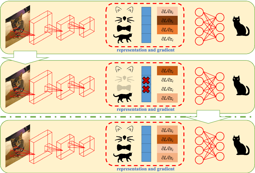
作者提出的方法是 Representation Self Challenging (RSC)，即将梯度高的认为是关键信息将其抹去来使模型学习更多的信息增强其泛化性能。

Method

RSC 主要有三步：

定位：首先计算前一层对应特征的梯度

\[ \begin{aligned} \mathbf {g}_\mathbf {z}= \partial (h(\mathbf {z};\widehat{\theta }_t^\text {top})\odot \mathbf {y})/\partial \mathbf {z}, \end{aligned} \]

其中 \(\odot\) 表示逐元素乘法，\(h\) 表示部分网络，\(x, y\) 表示输入和标签，RSC 计算 \((100-p)^{th}\) 的百分比的元素记为 \(q_p\) 然后得到一个掩模矩阵：

\[ \begin{aligned} \mathbf {m}(i) = {\left\{ \begin{array}{ll} 0, \quad \text {if}\quad \mathbf {g}_\mathbf {z}(i) \ge q_p \\ 1, \quad \text {otherwise} \end{array}\right. } \end{aligned} \]

掩模：使用掩模矩阵对特征 \(z\) 进行掩模 \(\begin{aligned} \tilde{\mathbf {z}}= \mathbf {z}\odot \mathbf {m} \end{aligned}\)
更新：计算 \(\begin{aligned} \tilde{\mathbf {s}} = \text {softmax}(h(\tilde{\mathbf {z}};\widehat{\theta }_t^\text {top})), \end{aligned}\) 然后使用梯度 \(\begin{aligned} \tilde{\mathbf {g}}_\theta = \partial l(\tilde{\mathbf {s}}, \mathbf {y})/\partial \widehat{\theta }_t \end{aligned}\) 更新模型

具体算法如下图所示

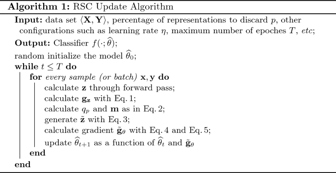
其实也不难理解，用通俗一点的语言解释：

先正常前向传播得到模型输出，然后反传计算中间层的特征梯度，根据梯度大小将确定一个 01 掩模矩阵

使用掩模矩阵对特征进行掩模然后重新前向传播得到输出

使用新的输出反传计算梯度更新模型

Detail

协变量偏移：每个域都相同的，例如猫的语义，但因为边缘分布的不同，可能会学习到不同的特征，例如尖尖的耳朵和胡须。

具体推论行文看得眼花缭乱，不看惹

有两种设置：逐空间的 RSC 和逐通道的 RSC

有 dropout 的衍生方法声称在训练的开始阶段不进行 dropout 操作，而是等网络学习到一定的特征以后再进行，作者也用上了有一点改进

Experiment

数据集：PACS, VLCS, Office-Home, ImageNet-Sketch

在使用其开源代码复现时发现其实是多源域泛化，例如在 PACS 中用其中一个域作为目标域而另外三个域合并作为源域

好吧，这一点翻回去看论文的时候发现论文里面也有提到

下面几个都是在 PACS 的消融实验

表1：逐空间的 RSC，drop 比例为 50%

Feature Drop Strategies	Backbone	Artpaint	Cartoon	Sketch	Photo	Avg ↑↑
Baseline [4]	ResNet18	78.96	73.93	70.59	96.28	79.94
Random	ResNet18	79.32	75.27	74.06	95.54	81.05
Top-Activation	ResNet18	80.31	76.05	76.13	95.72	82.03
Top-Gradient	ResNet18	81.23	77.23	77.56	95.61	82.91

表2：逐空间的 RSC，用了“Top-gradient"

Feature Dropping Percentage	Backbone	Artpaint	Cartoon	Sketch	Photo	Avg ↑↑
66.7%	ResNet18	80.11	76.35	76.24	95.16	81.97
50.0%	ResNet18	81.23	77.23	77.56	95.61	82.91
33.3%	ResNet18	82.87	78.23	78.89	95.82	83.95
25.0%	ResNet18	81.63	78.06	78.12	96.06	83.46
20.0%	ResNet18	81.22	77.43	77.83	96.25	83.18
13.7%	ResNet18	80.71	77.18	77.12	96.36	82.84

表3：逐空间的 RSC，用了“Top-gradient"，drop 比例调整为 33.3%

Batch Percentage	Backbone	Artpaint	Cartoon	Sketch	Photo	Avg ↑↑
50.0%	ResNet18	82.87	78.23	78.89	95.82	83.95
33.3%	ResNet18	82.32	78.75	79.56	96.05	84.17
25.0%	ResNet18	81.85	78.32	78.75	96.21	83.78

表4：“Top-Gradient”, Feature Dropping Percentage(33.3%33.3%) and Batch Percentage(33.3%33.3%).

Method	Backbone	Artpaint	Cartoon	Sketch	Photo	Avg ↑↑
Spatial	ResNet18	82.32	78.75	79.56	96.05	84.17
Spatial+Channel	ResNet18	83.43	80.31	80.85	95.99	85.15

表5：Ablation study of Dropout methods. “S” and “C” represent spatial-wise and channel-wise respectively. For fair comparison, results of above methods are report at their best setting and hyperparameters. RSC used the hyperparameters selected in above ablation studies:“Top-Gradient”, Feature Dropping Percentage (33.3%33.3%) and Batch Percentage (33.3%33.3%).

Method	Backbone	Artpaint	Cartoon	Sketch	Photo	Avg ↑↑
Baseline [4]	ResNet18	78.96	73.93	70.59	96.28	79.94
Cutout [6]	ResNet18	79.63	75.35	71.56	95.87	80.60
DropBlock [9]	ResNet18	80.25	77.54	76.42	95.64	82.46
AdversarialDropout [21]	ResNet18	82.35	78.23	75.86	96.12	83.07
Random(S+C)	ResNet18	79.55	75.56	74.39	95.36	81.22
Top-Activation(S+C)	ResNet18	81.03	77.86	76.65	96.11	82.91
RSC: Top-Gradient(S+C)	ResNet18	83.43	80.31	80.85	95.99	85.15

表6：DG results on PACS [13] (Best in bold).

PACS	Backbone	Artpaint	Cartoon	Sketch	Photo	Avg ↑↑
Baseline [4]	AlexNet	66.68	69.41	60.02	89.98	71.52
Hex [31]	AlexNet	66.80	69.70	56.20	87.90	70.20
PAR [30]	AlexNet	66.30	66.30	64.10	89.60	72.08
MetaReg [1]	AlexNet	69.82	70.35	59.26	91.07	72.62
Epi-FCR [14]	AlexNet	64.70	72.30	65.00	86.10	72.00
JiGen [4]	AlexNet	67.63	71.71	65.18	89.00	73.38
MASF [7]	AlexNet	70.35	72.46	67.33	90.68	75.21
RSC (ours)	AlexNet	71.62	75.11	66.62	90.88	76.05
Baseline [4]	ResNet18	78.96	73.93	70.59	96.28	79.94
MASF [7]	ResNet18	80.29	77.17	71.69	94.99	81.03
Epi-FCR [14]	ResNet18	82.10	77.00	73.00	93.90	81.50
JiGen [4]	ResNet18	79.42	75.25	71.35	96.03	80.51
MetaReg [1]	ResNet18	83.70	77.20	70.30	95.50	81.70
RSC (ours)	ResNet18	83.43	80.31	80.85	95.99	85.15
Baseline [4]	ResNet50	86.20	78.70	70.63	97.66	83.29
MASF [7]	ResNet50	82.89	80.49	72.29	95.01	82.67
MetaReg [1]	ResNet50	87.20	79.20	70.30	97.60	83.60
RSC (ours)	ResNet50	87.89	82.16	83.35	97.92	87.83

表7：DG results on VLCS [27] (Best in bold).

VLCS	Backbone	Caltech	Labelme	Pascal	Sun	Avg ↑↑
Baseline [4]	AlexNet	96.25	59.72	70.58	64.51	72.76
Epi-FCR [14]	AlexNet	94.10	64.30	67.10	65.90	72.90
JiGen [4]	AlexNet	96.93	60.90	70.62	64.30	73.19
MASF [7]	AlexNet	94.78	64.90	69.14	67.64	74.11
RSC (ours)	AlexNet	97.61	61.86	73.93	68.32	75.43

表8：DG results on Office-Home [28] (Best in bold).

Office-Home	Backbone	Art	Clipart	Product	Real	Avg ↑↑
Baseline [4]	ResNet18	52.15	45.86	70.86	73.15	60.51
JiGen [4]	ResNet18	53.04	47.51	71.47	72.79	61.20
RSC (ours)	ResNet18	58.42	47.90	71.63	74.54	63.12

表9：DG results on ImageNet-Sketch [30].

ImageNet-Sketch	Backbone	Top-1 Acc ↑↑	Top-5 Acc ↑↑
Baseline [31]	AlexNet	12.04	24.80
Hex [31]	AlexNet	14.69	28.98
PAR [30]	AlexNet	15.01	29.57
RSC (ours)	AlexNet	16.12	30.78

Conclusion

作者引入了一种简单的训练启发式方法，可以直接应用于几乎任何CNN架构，无需额外的模型架构，也几乎不需要增加计算工作量。作者将其命名为 RSC 。RSC 迭代地强制 CNN 在训练域中激活不太占主导地位但仍与标签相关的特征。RSC的理论和实证分析验证了RSC是扩展训练域特征分布的基础而有效的方法。

Code

看看作者给出的开源代码叭~

关键部分在模型的前向传播部分（略去了部分不太关心的模型函数）

class ResNet(nn.Module):
    def __init__(self, block, layers, jigsaw_classes=1000, classes=100):
        self.inplanes = 64
        super(ResNet, self).__init__()
        self.conv1 = nn.Conv2d(3, 64, kernel_size=7, stride=2, padding=3,
                               bias=False)
        self.bn1 = nn.BatchNorm2d(64)
        self.relu = nn.ReLU(inplace=True)
        self.maxpool = nn.MaxPool2d(kernel_size=3, stride=2, padding=1)
        self.layer1 = self._make_layer(block, 64, layers[0])
        self.layer2 = self._make_layer(block, 128, layers[1], stride=2)
        self.layer3 = self._make_layer(block, 256, layers[2], stride=2)
        self.layer4 = self._make_layer(block, 512, layers[3], stride=2)
        self.avgpool = nn.AvgPool2d(7, stride=1)
        # self.jigsaw_classifier = nn.Linear(512 * block.expansion, jigsaw_classes)
        self.class_classifier = nn.Linear(512 * block.expansion, classes)
        #self.domain_classifier = nn.Linear(512 * block.expansion, domains)
        self.pecent = 1/3

    def forward(self, x, gt=None, flag=None, epoch=None):
        x = self.conv1(x)
        x = self.bn1(x)
        x = self.relu(x)
        x = self.maxpool(x)

        x = self.layer1(x)
        x = self.layer2(x)
        x = self.layer3(x)
        x = self.layer4(x)

        if flag:
            interval = 10
            if epoch % interval == 0:
                self.pecent = 3.0 / 10 + (epoch / interval) * 2.0 / 10

            self.eval()
            x_new = x.clone().detach()
            x_new = Variable(x_new.data, requires_grad=True)
            x_new_view = self.avgpool(x_new)
            x_new_view = x_new_view.view(x_new_view.size(0), -1)
            output = self.class_classifier(x_new_view)
            class_num = output.shape[1]
            index = gt
            num_rois = x_new.shape[0]
            num_channel = x_new.shape[1]
            H = x_new.shape[2]
            HW = x_new.shape[2] * x_new.shape[3]
            one_hot = torch.zeros((1), dtype=torch.float32).cuda()
            one_hot = Variable(one_hot, requires_grad=False)
            sp_i = torch.ones([2, num_rois]).long()
            sp_i[0, :] = torch.arange(num_rois)
            sp_i[1, :] = index
            sp_v = torch.ones([num_rois])
            one_hot_sparse = torch.sparse.FloatTensor(sp_i, sp_v, torch.Size([num_rois, class_num])).to_dense().cuda()
            one_hot_sparse = Variable(one_hot_sparse, requires_grad=False)
            one_hot = torch.sum(output * one_hot_sparse)
            self.zero_grad()
            one_hot.backward()
            grads_val = x_new.grad.clone().detach()
            grad_channel_mean = torch.mean(grads_val.view(num_rois, num_channel, -1), dim=2)
            channel_mean = grad_channel_mean
            grad_channel_mean = grad_channel_mean.view(num_rois, num_channel, 1, 1)
            spatial_mean = torch.sum(x_new * grad_channel_mean, 1)
            spatial_mean = spatial_mean.view(num_rois, HW)
            self.zero_grad()

            choose_one = random.randint(0, 9)
            if choose_one <= 4:
                # ---------------------------- spatial -----------------------
                spatial_drop_num = math.ceil(HW * 1 / 3.0)
                th18_mask_value = torch.sort(spatial_mean, dim=1, descending=True)[0][:, spatial_drop_num]
                th18_mask_value = th18_mask_value.view(num_rois, 1).expand(num_rois, 49)
                mask_all_cuda = torch.where(spatial_mean > th18_mask_value, torch.zeros(spatial_mean.shape).cuda(),
                                            torch.ones(spatial_mean.shape).cuda())
                mask_all = mask_all_cuda.reshape(num_rois, H, H).view(num_rois, 1, H, H)
            else:
                # -------------------------- channel ----------------------------
                vector_thresh_percent = math.ceil(num_channel * 1 / 3.2)
                vector_thresh_value = torch.sort(channel_mean, dim=1, descending=True)[0][:, vector_thresh_percent]
                vector_thresh_value = vector_thresh_value.view(num_rois, 1).expand(num_rois, num_channel)
                vector = torch.where(channel_mean > vector_thresh_value,
                                     torch.zeros(channel_mean.shape).cuda(),
                                     torch.ones(channel_mean.shape).cuda())
                mask_all = vector.view(num_rois, num_channel, 1, 1)

            # ----------------------------------- batch ----------------------------------------
            cls_prob_before = F.softmax(output, dim=1)
            x_new_view_after = x_new * mask_all
            x_new_view_after = self.avgpool(x_new_view_after)
            x_new_view_after = x_new_view_after.view(x_new_view_after.size(0), -1)
            x_new_view_after = self.class_classifier(x_new_view_after)
            cls_prob_after = F.softmax(x_new_view_after, dim=1)

            sp_i = torch.ones([2, num_rois]).long()
            sp_i[0, :] = torch.arange(num_rois)
            sp_i[1, :] = index
            sp_v = torch.ones([num_rois])
            one_hot_sparse = torch.sparse.FloatTensor(sp_i, sp_v, torch.Size([num_rois, class_num])).to_dense().cuda()
            before_vector = torch.sum(one_hot_sparse * cls_prob_before, dim=1)
            after_vector = torch.sum(one_hot_sparse * cls_prob_after, dim=1)
            change_vector = before_vector - after_vector - 0.0001
            change_vector = torch.where(change_vector > 0, change_vector, torch.zeros(change_vector.shape).cuda())
            th_fg_value = torch.sort(change_vector, dim=0, descending=True)[0][int(round(float(num_rois) * self.pecent))]
            drop_index_fg = change_vector.gt(th_fg_value).long()
            ignore_index_fg = 1 - drop_index_fg
            not_01_ignore_index_fg = ignore_index_fg.nonzero()[:, 0]
            mask_all[not_01_ignore_index_fg.long(), :] = 1

            self.train()
            mask_all = Variable(mask_all, requires_grad=True)
            x = x * mask_all

        x = self.avgpool(x)
        x = x.view(x.size(0), -1)
        return self.class_classifier(x)

好像有一点点复杂，不看惹~

结果复现

使用开源代码在 PACS 进行结果复现

根据个人所使用的服务器的情况对代码的一些部分进行了微调

原论文中结果在后面括号备注 RSC，复现结果在后面括号备注 Ours.

因为服务器比较拥挤，没有足够的显存，所以 ResNet50 的复现结果中 batch size 减小到 32 (默认值为 64 预计需要显存 15 G左右)

后面发现不知道为什么结果差太远了想办法协商了下跑了 64 的 batch size 发现结果相差极大

Method	Backbone	Art painting	Cartoon	Sketch	Photo	Avg
Baseline(RSC)	ResNet18	78.96	73.93	70.59	96.28	79.94
RSC(RSC)	ResNet18	83.43	80.31	80.85	95.99	85.51
RSC(Ours)	ResNet18	79.79	80.67	82.74	93.83	84.26
Baseline(RSC)	ResNet50	86.20	78.70	70.63	97.66	83.29
RSC(RSC)	ResNet50	87.89	82.16	83.35	97.92	87.83
RSC(Ours, bs32)	ResNet50	77.24	82.03	82.69	93.71	83.91
RSC(Ours, bs64)	ResNet50	85.35	85.92	84.09	95.20	87.64
RSC(Ours*)	ResNet50	84.13	81.86	79.90	99.42	86.32

* 将开源代码中模型挪移到自己编写这边的框架来进行测试

References

如果对你有帮助的话，请给我点个赞吧~

欢迎前往我的博客查看更多笔记