Information
- Title: Spectral Normalization for Generative Adversarial Networks
- Author: Takeru Miyato, Toshiki Kataoka, Masanori Koyama, Yuichi Yoshida
- Institution: Preferred Networks, Inc.(PFN, 日本最大人工智能企业)
- Year: 2018
- Journal: ICLR
- Source: Arxiv, Official code, OpenReview, Other materials
- Idea: 利用 SN 约束鉴别器的 Lipschitz 常数稳定 GAN 的训练
1 | @inproceedings{miyato2018spectral, |
Abstract
提出了一种新的权重归一化方法,谱归一化(Spectral normalization), 用于在训练过程稳定鉴别器。这种方法很轻量而且很容易添加到已有的实现方法中,效果和一些已有的方法一样好甚至犹有过之。
Introduction
训练 GAN 网络的一个难点是控制鉴别器的性能,设想一下,如果鉴别器太优秀了,那么分类器的训练就会陷入停滞,因为其导数变成 0 了,这启示着我们要对鉴别器做一些限制。
这篇文章提出了称为 Spectral normalization 的权重归一化方法,用于在训练中稳定鉴别器。其优点是
- 仅 Lipschitz 常数一个超参数,而且这个超参数也不怎么需要调整
- 实现简单计算代价小
Method
鉴别器可以表示为 $$ D(x, \theta) = {\rm \mathcal{A}}(f(x, \theta)) $$ 𝒜 表示激活函数,而 GAN 的目标函数为: minGmaxDV(G, D) 而 V 由下式给出 $$ \mathrm{E}_{x\sim q_{\rm data}} [\log D(x)] + \mathrm{E}_{x'\sim p_G} [\log(1-D(x'))] $$ 其中 $ q_{}$ 是数据分布而 pG 是生成分布,那么对于固定的生成器 G , 鉴别器的优化目标为 $$ D^*_G(x) := \dfrac{q_{\rm data}(x)}{(q_{\rm data}(x) + p_{G}(x))} $$ 最近一些工作指出鉴别器的函数空间对于 GAN 的性能至关重要,有许多工作也提出 Lipschitz 连续在统计有界的重要性。,例如: $$ D_{G}^*(x) = \frac{q_{\rm data}(x)}{q_{\rm data}(x)+p_G(x)} = {\rm sigmoid}(f^*(x)), \text{where }f^*(x) = \log q_{\rm data}(x) - \log p_G(x) $$ 其导数 $$ \nabla_x f^*(x) = \frac{1}{q_{\rm data}(x)}\nabla_{x}q_{\rm data}(x) - \frac{1}{p_G(x)}\nabla_{x}p_G(x) $$ 可能是无穷大或无法计算,这启示着我们对 f(x) 的导数引入一些正则化条件。
Spectral Normalization
谱归一化(Spectral Normalization) 通过约束每层 g : hin ↦ hout 的谱范数来控制鉴别器函数 f 的 Lipschitz 常数。Lipschitz 范数 $\|g\|_{\rm Lip}$ 等价于 suphσ(∇g(h)),其中 σ(A) 是矩阵 A 的谱范数(A 的 L2 矩阵范数): $$ \sigma(A) := \max_{h: h \neq { 0}} \frac{\|Ah\|_2}{\|h\|_2} = \max_{\|h\|_2\leq 1} \|Ah\|_2 $$ 同样等于 A 的最大奇异值。对于线性层 g(h) = Wh 其范数为 $|g|_{} = _h (g(h)) = _h (W) = (W) $. 如果激活函数的 $\|a_l\|_{\rm Lip}$ 等于 1,那么可以根据不等式 $\|g_1\circ g_2\|_{\rm Lip}\leq\|g_1\|_{\rm Lip}\cdot\|g_2\|_{\rm Lip}$ 得到 $\|f\|_{\rm Lip}$ 的上界: $$ \begin{align} \|f\|_{\rm Lip} \leq & \|(h_{L}\mapsto W^{L+1}h_{L})\|_{\rm Lip}\cdot \|a_L\|_{\rm Lip}\cdot\|(h_{L-1}\mapsto W^ Lh_{L-1})\|_{\rm Lip} \nonumber \\ &\cdots \|a_1\|_{\rm Lip}\cdot\|(h_0\mapsto W^ 1h_0)\|_{\rm Lip} = \prod_{l=1}^{L+1} \|(h_{l-1}\mapsto W^lh_{l-1})\|_{\rm Lip} = \prod_{l=1}^{L+1} \sigma(W^l). \end{align} $$ Spectral Normalization 对权重矩阵 W 的谱范数做归一化使其满足 Lipschitz 约束 σ(W) = 1: $$ \bar{W}_{\rm SN}(W) := W / \sigma(W) $$
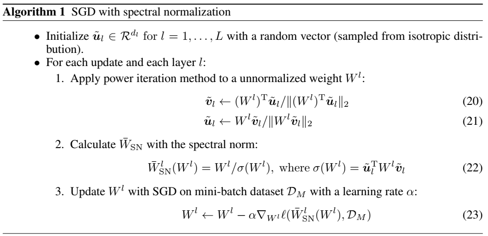
Fast Approximation
简单来说就是计算奇异值的计算开销太大了,所以作者借鉴另一篇文章提出使用迭代的方法来估算奇异值
Gradient Analysis
$\bar{W}_{\rm SN}(W)$ 的梯度是: $$ \frac{\partial \bar{W}_{\rm SN}(W)}{\partial W_{ij}} = \frac{1}{\sigma(W)}E_{ij} - \frac{1}{\sigma(W)^2} \frac{\partial \sigma(W)}{\partial W_{ij}} W =\frac{1}{\sigma(W)}E_{ij} - \frac{[u_{1}v_{1}^{\rm T}]_{ij}} {\sigma(W)^2} W = \frac{1}{\sigma(W)}\left(E_{ij} - [u_{1}v_{1}^{\rm T}]_{ij} \bar{W}_{\rm SN}\right) $$ 鉴别器的梯度为: $$ \begin{align} \frac{\partial V(G,D)}{\partial W} &= \frac{1}{\sigma(W)} \left(\hat{\rm E}\left[\delta h^{\rm T}\right] - \left(\hat{\rm E}\left[\delta^{\rm T} \bar{W}_{\rm SN}h \right] \right) u_1 v_1^{\rm T} \right) \\ &=\frac{1}{\sigma(W)} \left(\hat{\rm E}\left[\delta h^{\rm T}\right] - \lambda u_1 v_1^{\rm T} \right) \label{eq:grad_sn} \end{align} $$ 其中 $\delta := \left(\partial V(G,D) / \partial \left(\bar{W}_{\rm SN} h\right)\right)^{\rm T}$, $\lambda:=\hat{\rm E}\left[\delta^{\rm T} \left( \bar{W}_{\rm SN}h \right)\right]$. $\hat{\rm E}[\cdot]$ represents empirical expectation over the mini-batch. $\frac{\partial V}{\partial W}=0$ when $\hat{\rm E}[\delta h^{\rm T}] = ku_1 v_1^T$ for some k ∈ ℝ.
这段没太看懂
Compare
主要是与 Weight Normalization 的对比,大意是 WN 抑制了鉴别器的性能,其约束太强了。因为 WN 等价于 $$ \sigma_1(\bar{W}_{\rm WN})^2 + \sigma_2(\bar{W}_{\rm WN})^2 + \cdots + \sigma_T(\bar{W}_{\rm WN})^2 = d_o,~{\rm where}~T=\min(d_i,d_o) $$ 而 Lipschitz 常数值取决于最大的奇异值。
orthonormal regularization 通过 $$ \|W^{\rm T} W-I\|_F^2 $$ 将所有奇异值设置为1而 SN 只是将最大特征值设置为1
Experiment
注意到对于卷积核的处理是将 $W \in \mathbb{R}^{d_{\rm out}\times d_{\rm in} \times h \times w}$ 的卷积核化为 $d_{\rm out}\times (d_{\rm in} h w)$ 形状进行处理。
Conclusion
首先,提出了 Spectral normalization 的方法,该方法用于稳定 GANs 的训练,该方法比传统的 Weight normalization 的方法生成的图像更加多样化,并且IS比先前的工作要更优。该方法使用了全局正则化的方法,但也可以和局部正则化的方法联合使用。作者后续的工作将进一步研究更多的理论基础,已经在更大更复杂的数据集上使用。
文章大意是基本上看明白了,但为什么这么做和这么做有什么用其实还是一知半解,主要原因还是对 GAN 了解不是很深入,GAN 的一些问题和关键都不太了解导致的。
References
如果对你有帮助的话,请给我点个赞吧~
欢迎前往 我的博客 查看更多笔记